We tackle the problem of Federated Learning in the non i.i.d. case, in which local models drift apart, inhibiting learning. Building on an analogy with Lifelong Learning, we adapt a solution for catastrophic forgetting to Federated Learning. We add a penalty term to the loss function, compelling all local models to converge to a shared optimum. We show that this can be done efficiently for communication (adding no further privacy risks), scaling with the number of nodes in the distributed setting. Our experiments show that this method is superior to competing ones for image recognition on the MNIST dataset.
This is the first, introductory post, in our three part algorithmic series on real-world distributed training on the edge. In it, we present and compare the two fundamental methods for this type of machine learning (and Deep Learning in particular). The post following this one will then address communication compression, and the final one will attend to the challenge that non-IID distributions pose, specifically for Batch Normalization.
Distributed Edge Training
With the increased penetration and proliferation of IoT devices, and the continuous increase in connected, everyday devices (from smartphones to cars to self check out stands), the amount of data collected from the world is increasing exponentially. Against this, there are:
Growing privacy concerns, and the security risks associated with access to so much data.
Costs or constraints on transmitting all that data for training purposes.
A question presents itself: With all of the data generated on these edge devices, and with those devices having more processing power than ever before — does the data really need to leave the device? Why not just have the training process itself run on the edge device? This, to be sure, goes well beyond the commonly used term “AI at the edge”, which usually refers to the use of local models (that merely make predictions on the device).
Now, a single edge device still offers a highly limited amount of collected data and packs relatively little computational power. But in many contexts there is a multitude of them that are performing very similar training tasks. If these could all collaborate between them, and together train a shared model, one that gains from the vast data collected from all of them, it would be a whole new ball game. And if this could be done while keeping the data on the devices themselves (as they are the ones who carry out the training anyway), it would decouple the ability to train the shared model from the need to store the data in a datacenter.
This would be nothing short of a revolution for AI privacy.
A new generation of algorithms for training deep learning models, that do just that, is emerging. This is what we term Distributed Edge Training, bringing the model’s training process to the edge device, while collaborating between the various devices to reach an optimized model. For a more product/solution- oriented overview, see our initial post on the topic. Here, we attend to the algorithmic core of these methods.
The Basic Idea and Its Challenges
Our goal is to train a high-quality model while the training data remains distributed over a large number of edge devices. This is done as follows:
The instances of learning algorithms running on the edge devices, all rely on a shared model for their training. In a series of rounds, each device, after downloading the current model (or what it takes to deduce it), independently computes some form of update to that model based on its local data. It communicates this update back to the server, where the updates are then aggregated to compute a new global model. During the process, the training data remains on the edge devices.
We will explore and compare two of the most common approaches for powering Distributed Edge Training: Federated Learning (as promoted first and foremost by Google) and Large Batch Learning (see also here) (by Facebook and others) {originally suggested for fast training on hyper computing clusters.}
Though the idea behind Distributed Edge Training is conceptually simple, it can get technically complex. These approaches are efficient in some scenarios, but have proven to be much more challenging in others, depending on various factors:
The number of concurrent edge devices that impact the shared model (where a large number of endpoints can hinder performance)
The distribution of data among those endpoints (where an uneven, non IID fashion presents a deep challenge to such approaches)
Network bandwidth limitations (where not all approaches lend themselves to compression schemes equally)
We have set out to evaluate Federated Learning and Large Batch with respect to these factors and others. The next two posts, specifically, will revolve around points 2 and 3 respectively.
For presentation’s sake, we will be making a number of simplifying assumptions:
All communication between the edge devices is done through a single, central server.
Synchronised Algorithms — a simple implementation of the distribution framework. It requires that each device sends a model or model gradients (or model update) back to the server during each round.
The Machine Learning algorithmic framework is that of Deep Learning (other methods also lend themselves to such distribution schemes).
Furthermore, the Deep Learning training uses a standard optimizer — Stochastic Gradient Descent (SGD).
Large Batch
In classical, non-distributed batch training, a batch of samples is used in order to perform a stochastic gradient descent optimization step. With large batches allowed for (With large batches allowed for — which is not always simple or even feasible), it is rather straightforward for this process to be a distributed one, running over many server GPUs or, in our case, edge devices:
While each edge device has its own local data, that can be considered as part of the batch. Each device, performing a forward and backward pass on its data, calculates a single local gradient each time. The calculated gradient is then sent to the server, where these are all aggregated, for the sake of a global update to the model. (The aggregate or the updated model are sent back to the devices, and the cycle repeats.)
To spell out the Large Batch steps:
Initialise the weights for the shared model. — — — — — — — — edge device phase — — — — — — — —
Download the current shared model.
Run a single pass of forward prediction and backward error propagation.
Compress the gradients.
Upload the update to a central server. — — — — — — — — server phase — — — — — — — —
Decompress the incoming gradients and compute their average
Perform a single step of SGD to update the shared model.
Go to step 2 (edge training phase).
Federated Learning
In Large Batch, in every round, each device performs a single forward-backward pass, and immediately communicates the gradient. In Federated Learning, in contrast, in every round, each edge device performs some independent training on its local data (that is, without communicating with the other devices), for several iterations. Only then does it send its model-update to the server to be aggregated with those of the other devices, for the sake of an improved shared model (from which this process can then repeat).
Here, too, during the whole process, all of the training data remains on the devices.
To spell out the Federated Learning steps:
Initialise the weights for the shared model. — — — — — — — — edge device phase — — — — — — — —
Download the current shared model.
Run a number of SGD iterations (based on forward and backward passes upon the local data).
Compress the updated model weights (optional).
Upload the update to the central server. — — — — — — — — server phase — — — — — — — —
Decompress the incoming weights of the machines’ models if needed.
Compute their average.
Update the shared model.
Go to step 2 (edge training phase).
The Two Approaches in Comparison
Without the multi-stage device independent training of Federated Learning, distributed Large Batch training is more similar to classical training, in which the data resides in one central location. The average of gradients of local batches is equivalent to an average of the gradients of all the samples in the large batch, which is exactly what happens in standard SGD training. The only thing that breaks the equivalence are the local data-dependent transformations such as batch normalization. The batch normalization is performed over each local batch separately instead of over the entire large batch combined.
Being the more radical approach, means that Federated Learning encounters some unique challenges. Perhaps the most crucial one concerns the distribution of data among the edge devices. For Federated Learning to achieve good performance, the classes distribution needs to be as similar as possible across the devices. For highly uneven, non-IID distributions of the local datasets (a rather common situation), Federated Learning performance deteriorates.
Federated learning has a hard time handling batches that are unevenly distributed
Large Batch, in comparison, is far better equipped to handle data which is non IID distributed: The averaging of the gradient over the local batches smoothes out the distribution. The large averaged batches are IID, or at least more so than the small local ones.
With this and the other challenges that Federated Learning brings with it, running independent multi-stage training has the clear, direct advantage of requiring fewer client-server communications. Fewer than in Large Batch training, that is, where communication has to occur constantly, with every batch. (On the other hand, being able to send out gradients instead of actual weights, does allow for some sparsity-based compression techniques to be applied.)
A Preliminary Empirical Comparison
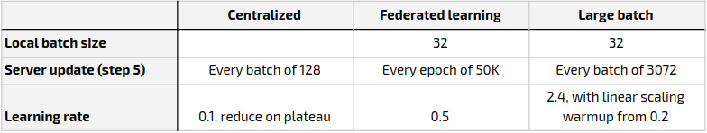
We have set out to benchmark the two approaches, pinning them against each other and against classical, single-server training. Our basic comparative philosophy was to run each methodology according to its own fitting or “standard” parameters, to the extent that this is possible. Large Batch requires comparably larger learning rates, for example, and so simply using the same parameters across all methodologies wouldn’t do. On the other hand, for the by-epoch comparison to make any kind of sense, we had to keep some uniformity. Importantly, as using momentum didn’t fit our optimization of the Federated Learning run, we had to avoid using momentum for the centralised and Large Batch training as well.
The experiment settings were as follows:
Dataset: CIFAR10, a relatively small, widely used benchmarking dataset. The 60K data points were split into a training set of 50K and a testing set of 10K data points. (We will present experiments on more substantial datasets in future posts.)
Architecture: Resnet18 (a common deep learning architecture). Training was done from scratch (no pre-training).
Optimizer: SGD
Distributed setting: The training process was distributed across 96 virtual CPUs (with Intel Skylake inside). The training data for this experiment (before we get to post 3) was distributed in an even (IID) fashion.
Table 1: The parameters of the different methods
The experiment results were as follows (figure 1):
Figure 1: A graph of the three compared approaches — Large Batch, Federated Learning, and the classic single-server SGD training.
Using larger batches can slow convergence, as can more “extreme federating” of the training (synchronising once every more training rounds). In more challenging settings these can certainly also hurt or even destroy the final accuracy, though in the experiment above both distributed approaches managed to come close to the accuracy level of standard centralised training — ultimately. But as for speed, purely in terms of the epochs (i.e. passes on the data), the classical centralised approach indeed came out the fastest (with Federated Learning a far third).
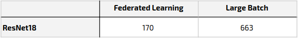
Convergence by number of epochs, however, is in itself beside the point. The settings we are interested in are distributed to begin with. In those, training time is not simply computation time, but can be critically constrained by the communication cost. That, in turn, is intimately tied to the number of communication rounds. And after all, this was the point of developing Federated Learning over the more-standard Large Batch distribution. How do these two approaches compare in that fundamental respect, then? Here is a summary of the number of rounds required for reaching 80% accuracy in the experiment above:
Table 2: Number of communication rounds required during the training in order to reach an accuracy of 80% in the experiment as above. For Federated Learning, synched once every epoch, this is simply the number of epochs for 80% accuracy. For Large Batch, this is the number of epochs for 80% accuracy, times the number of (3072) batches that go into a single epoch (of 50,000 samples).
Conclusion
Distributing the training among many edge devices provides groundbreaking advantages. It also means, however, that communication cost now becomes an important factor, which has to be taken into account and managed, somehow. The number of rounds is but one fundamental aspect of it. The other side of the coin is the amount of data that has to be sent each time. This is the topic of our next post.
For now, to end on a very general note:
Our research, as we present here and in future posts, shows that there is no clear winner between the federated learning and Large batch approaches. Each has its pros and cons, depending mainly on the particulars of the use cases. Federated learning proves better for applications where connectivity is scarce and data is distributed uniformly (IID), whereas Large Batch fits better when data is distributed unevenly (Non IID) and communication is steady, and when we can gain value from high compression rates. Moreover, Federated Learning is only now beginning to be made to work for more complex problems such as the classification of Imagenet.
Our underlying recommendation is that researchers be proficient in both approaches and have the flexibility to choose between them according to the different use cases.
In the first post of this series, we presented two basic approaches to distributed training on edge devices. In the second, we explored compression methods for those approaches. Diving deeper into the real-world challenges of these training methodologies, we now introduce a problem with common architectures that arises from certain common data distributions — and the solution we have found for it.
Non IID Data Distribution
Training at the edge, where the data is generated, means that no data has to be uploaded to the cloud, thereby maintaining privacy. This also allows for continuous, ongoing training.
That being said, keeping things distributed, by its very nature, means that not all edge devices see or are privy to the same data sets. Take Amazon Go, for example. Their ceiling cameras capture different parts of the store, and hence different types of products. This means that each camera will have to train on a different dataset (and will therefore produce models at varying levels of quality).
In the distributed setting, then, there is no guarantee that the data will have identical distributions across the different devices. This presents a great challenge for schemes that rely on global statistics.
One such component which is extremely common in modern architectures, is that of a batch normalization layer. We show that batch norm is susceptible to non-IID data distribution and investigate alternatives. Our focus is on a distributed training setup with a large number of devices and hence a large batch training.
The Impact on Batch Normalization
Batch Normalization [1] layer performs normalization along the batch dimension, meaning that the mean and variance of each channel are calculated using all the images in the batch. Normalizing across the batch suffers inaccuracies when running prediction and the batch size reduces to 1. In order to address this, In prediction the layer uses mean and variance values that were aggregated over the entire data set during training. When training is distributed and each device has its own local data, the batch also becomes distributed and each device trains on a local batch before global aggregation. The normalization performed by Batch Normalization during training is on the local batch statistics while the running mean and average is aggregated globally. Thus, when the data is non identically distributed, the batch statistics of each device do not represent the global statistics of all the data, making the prediction different than the training. Training a deep neural network with batch normalization on non IID data is known to produce poor results [5].
Group Normalization to the Rescue
Group Normalization [3][4] is an alternative to Batch Normalization which does not use the “batch” dimension for normalization. It has been proposed for cases where normalizing along the batch dimension is not appropriate. For example, at inference time or when the batches are too small for accurate statistics estimation. Group Normalization works the same way for training and prediction. It divides the channels of each image into groups and calculates the per-group statistics for each image separately. Since the statistics are computed per-image, Group Normalization is completely invariant to the distribution of data across the workers, which makes it a suitable solution for non IID cases.
In the experiments section we investigate the effect of training Resnet using Group Normalization (in place of Batch Normalization) in a non-IID scenario. Our investigation focuses on training in a large batch scenario simulating a large number of machines. We show that as the batch size increases, the Group Normalization variant of Resnet shows an increasing degradation in validation accuracy. This could be attributed to Group Normalization losing some regularization ability in comparison to Batch Normalization [3]. We found similar degradation happening when using other normalization methods, such as Layer Normalization or Instance Normalization.
Training Without Normalization — Fixup Initialization
A recent paper [6] suggests that deep neural networks can be trained without layer normalization, by properly rescaling the weights initialization. The paper maintains that using common initializations leads to exploding gradients on very deep networks at the beginning of training. Similar to Batch Normalization, the paper also adds learned scalar multipliers and scalar biases to the neural network architecture. Using these changes to the weight initialization and the architecture, the authors were able to train Resnet without the use of batch normalization layers, achieving SOTA results. In what follows, we term the resulting network Resnet-Fixup.
In our experiments, training Resnet-Fixup using large batches shows sensitivity to increasing the learning rate, with training tending to suffer from exploding gradient when the learning rate is increased linearly with the batch size (as is commonly done [9]). However, we were able to train Resnet-Fixup with large batches on CIFAR10, achieving SOTA accuracy, using a carefully-tuned learning rate strategy, as we detail in the experiments section.
The Experiments
Non-IID
In order to simulate non-IID training on CIFAR10 (which has 10 classes), we used 10 devices for training, dividing the data so that each device gets images from only two classes. We trained with batch size of 320, using SGD, with a learning rate of 0.1, momentum of 0.9, and weight decay of 5e-4.
We trained using Vanilla Resnet18 on IID data as reference. All other networks were adaptations of Resnet18 for Group Normalization and Resnet-Fixup, as previously explained.
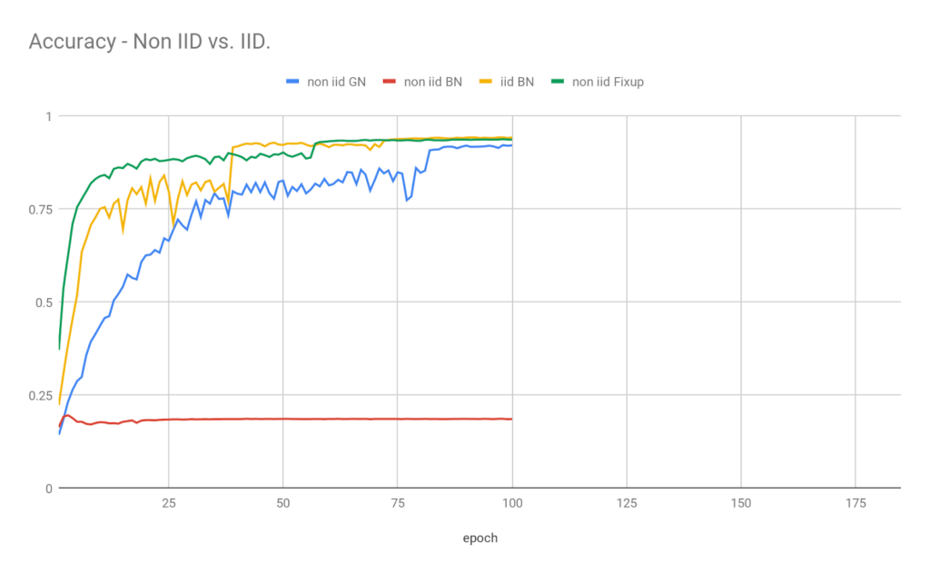
Figure 2 shows the results. We see that training Vanila Resnet18 in this non-IID scenario produces random predictions on validation. However, both Group Normalization and Resnet-Fixup are unaffected by the data distribution. The validation accuracy for group-norm Resnet18 on Non IID data is a bit lower than the IID case. This is the result of the loss in regularization when moving to Group-Normalization. Next we will see that the degradation in accuracy increases as the batch size is increased.
Figure 2: Validation accuracy of the IID and Non IID case. The reference (iid BN) is Vanilla Resnet18 trained on IID data. The rest are Resnet18 and variants of Resnet18 (GN for group norm and Fixup for Resnet-Fixup) trained on non IID data. While training with Batch-Norm leads to random results (non iid BN) Group Norm and Fixup resnets achieve accuracy similar to the IID batch-Norm scenario with Group Norm a bit lower.
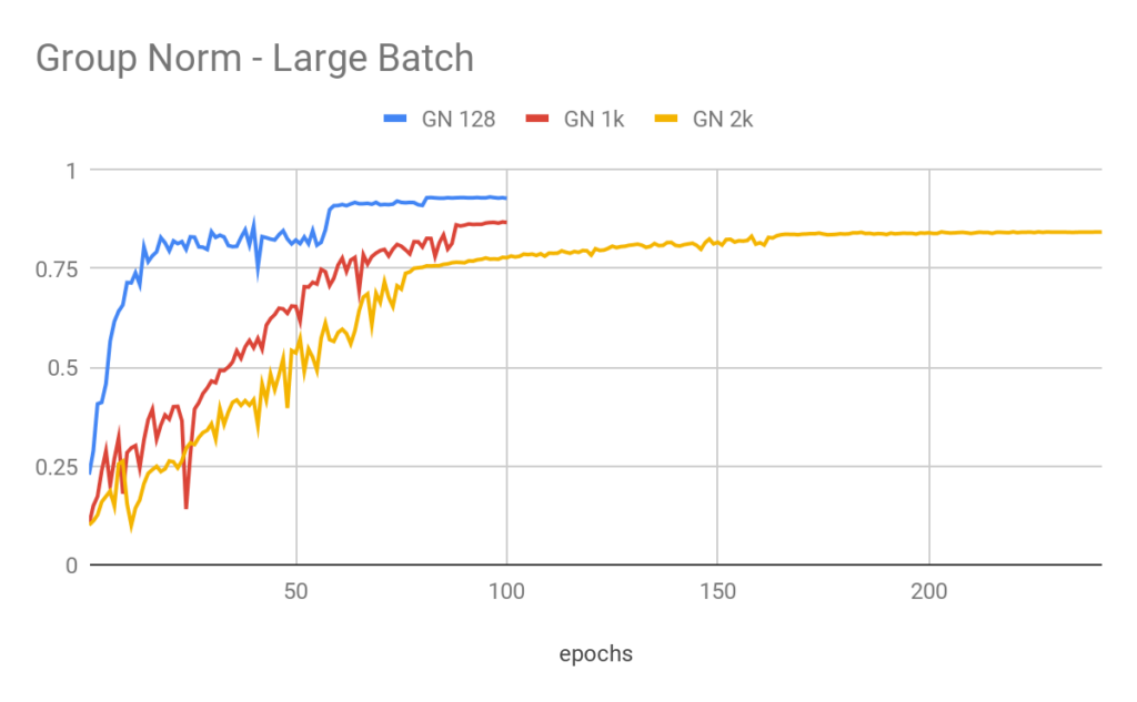
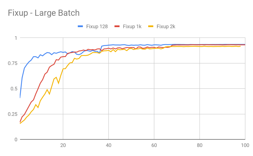
Large batch training
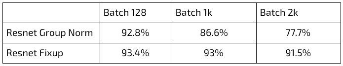
We examine the effect increasing the training batch size on our two solutions, namely Group Normalization and Fixup initialization. We train Resnet18 on CIFAR10 with batch size of 128, 1k, and 2k.
For Group Normalization, we used SGD with a learning rate of 0.1, momentum of 0.9, and weight decay of 5e-4. For the batch size 128, learning rate was reduced on plateau. For batch sizes 1k and 2k we used warmup to increase the learning rate linearly from 0.1 to 0.8 and 1.6 respectively over 6 epochs and then reduce learning rate on plateau.
For Fixup, we trained with SGD with momentum and weight decay as in the Group Norm case. Learning rate for the 128 baseline was 0.1 and then reduced on plateau. For the 1k and 2k cases, we experienced exploding gradient when we tried to increase the learning rate linearly with the batch size (as was done for Group Normalization). So we used warmup from 0.01 to 0.1 for the first 20 epochs and then reduce on plateau. Training Resnet Group-Normalization using this learning rate policy did not produce different results.
In Figure 4 we see that the Group Normalization Resnet accuracy degrades as the batch-size is increased. In Figure 5 we see that using Fixup initialization we were able to able to train with little loss of accuracy loss.
Results are summarized in table 1.
Validation accuracy for large batch training on CIFAR10 with Resnet18 after 100 epochs.
Figure 3: Validation accuracy for Resnet18 with Group Normalization on large batch training. Accuracy drops as batch size increases
Federated Learning
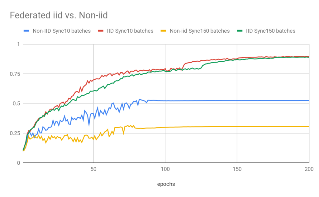
To conclude, we would like to address an additional challenge of training on non IID data with Federated Averaging. In the scenario described above where each device has data from different classes the models drift apart and suffer from catastrophic forgetting. This phenomena becomes more pronounced as the aggregation frequency is reduced.
We use the above Non-IID setup to train Resnet18 with group normalization layers using Federated Averaging. Each device has 5000 images, and the local batch size is 32. To test how synchronization frequency effects training, we synchronize the models by aggregation every 10 and every 150 batches.
Figure 3 shows the results of the non IID data against the IID case. We see that catastrophic forgetting reduces the validation accuracy to nearly 50% for the 10 batch synchronization frequency while when synchronization jumps to 150 batches devices only learn their local data.
Conclusion
The unconstrained nature of data distribution on the edge poses some major challenges for on the edge training. We showed that some of today’s most prolific neural network architectures fail when training on non IID data.
As we showed, architectures that do not use batch normalization entail searching for new hyper parameters for the training algorithms as well. This point is further aggravated when training with the Federated Averaging algorithms since non IID distribution causes catastrophic forgetting. We believe that new algorithms will need to be developed and this will be a matter for future research.
This series of articles regarding distributed learning was written by the Edgify research team. Feel free to join the conversation on the Federated learning facebook group!
In the first post of this series we presented two basic approaches to distributed training on edge devices (if you haven’t read our first post in this series, you should start here). These approaches provide benefits such as AI data privacy and the utilization of the compute power of edge devices. Large-scale distributed training systems, however, may fail to fully utilize that power (as we’ve come to see in our own experiments), as they consume large amounts of communication resources. As a result, limited bandwidth can impose a major bottleneck on the training process.
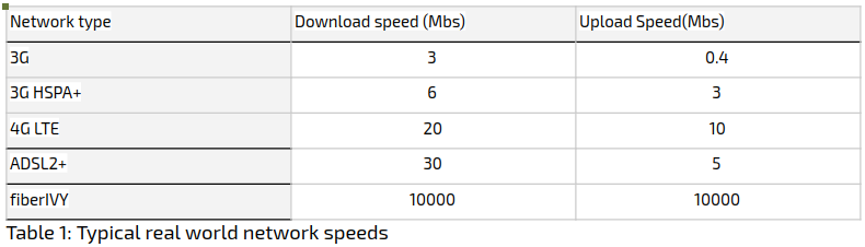
The two issues described below, pose additional challenges to the general limitation of bandwidth. The first has to do with how synchronized distributed training algorithms work: the slowest edge device (in terms of network bandwidth) “sets the tone” for the training speed, and such devices need to be attended to, at least heuristically. Secondly, the internet connection on edge devices is usually asymmetric, typically twice as slow for upload then for download (table 1). This can severely impede the speed of training when huge models/gradients are sent via the edge devices for synchronization.
Network resources are limited not only by the physical capacity of the underlying fiber/cable that carries the traffic, but also by the processing power and memory of the network devices (these devices/routers are responsible for the difficult task of routing traffic through the network). The network tends to congest when it carries more data than it can handle, which leads to a reduction in network performance (due to TCP packet delay/loss, queueing delays, and blocking of new connections).
Such network restrictions can significantly slow down the training time. In addition, the training must be robust to network failure in order to ensure a stable, congestion-free network. Moreover, in cases where network congestion occurs, the trainer needs to be able to handle it and resume the training process once the network is stable.
There are two main algorithmic strategies for dealing with the bandwidth limitation: (1) Reducing the number of communication rounds between the edge devices and the server (2) Reducing the size of the data transferred in each communication.
1) Reducing communication rounds, as described in the previous post:
Federated Learning is a paradigmatic example for reduced communication. Running Large Batch training requires a communication operation to occur with each batch. Federated Learning, in contrast, runs on the edge device for as many iterations as possible, thus synchronizing the models between the edges as little as possible. This approach is being researched widely in search of ways to reduce communication rounds without hurting accuracy.
2) Reducing the size of the data transferred in each communication, as we now detail in this post. To explain how this can be done, let us first recall the basics of the Large Batch and Federated Learning training methods.
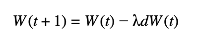
Deep Learning training uses a gradient based optimization procedure for the weights update. A standard procedure for this is Stochastic Gradient Descent (SGD), which can easily be adapted to Large Batch training. Formally, at communication iteration t the following update is performed :
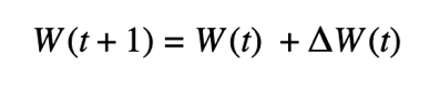
where dW(t) is the average of gradients across all devices and λ is the learning rate. One could also consider the weight update at communication iteration t for Federated Learning. This can be done as follows:
where ΔW(t) is the average of local updates across all devices. Namely, for device i at round t, ΔW(t) is the difference between the initial model for this round W(t) and the final local model Wᵢ(t+1) (the local model that the device sends for averaging at the end of the round). Although the model delta ΔW(t) is not a gradient.
The methods we explored for reducing the amount of data transfer are quantization and sparsification. We can apply those methods to the weights themselves, or to the gradients. We adapt the gradient compression methods to Federated Learning by applying those methods to the weight deltas instead of the gradients.
Gradient quantization (GQ)
GQ is a low precision representation of the gradients, which reduces the data transfer in each communication. So far, there has been limited research on the use of GQ. Some of the known methods of low-precision quantization are 1-bit SGD [1], QSGD [2], and TernGrad [3]. One of the most straightforward methods for quantization is “float32 to int8” (F2I), which reduces the amount of data by a factor of 4. F2I quantization is used widely in the context of inference; this method is integrated in some of the common deep learning frameworks (such as TensorFlow and Caffe) as part of their high performance inference suite. Our experiments show that quantizing the model weights for the training phase is a bad strategy. Quantizing the gradients (GQ), however, does produce good results in training.
Further data reduction can be achieved by using the standard Zip method on the quantized weights. Experiments we’ve conducted reached a reduction of about 50%.
Gradient Sparsification (GS)
Unlike quantization methods, where we try to preserve the information in the gradients with a low precision representation, in GS we try to figure out which parts of the gradients are actually redundant and can be ignored (which can prove to be quite a challenging task). Basic algorithms for GS drop out elements that are smaller than some predefined threshold. The threshold can be predefined before training, or can be chosen dynamically based on the gradient statistics. One such GS method is called “Deep Gradient Compression (DGC)” [4], which is essentially an improved version of “Gradient Sparsification”[5]. In DGC, the threshold is determined dynamically using the gradient statistics. The data that falls below the threshold is accumulated between communication rounds, until it is large enough to be transferred. The threshold is determined by the percentage of data one would like to send, using smart sampling (sampling only 1% of the gradients in order to estimate the threshold). DGC also employs momentum correction and local gradient clipping to preserve accuracy [4].
The Experiments
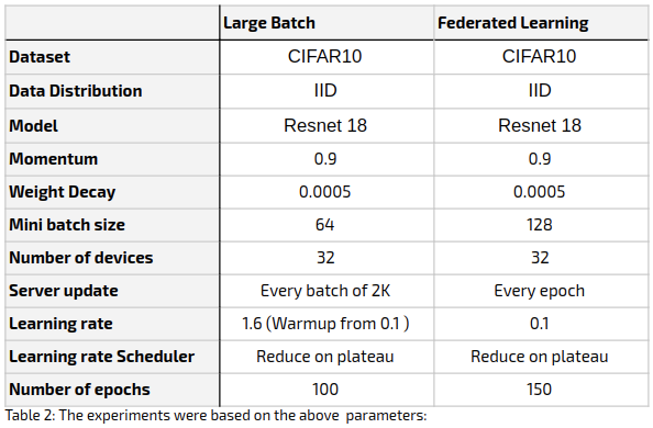
In our experiments, we have explored the possibility of applying these compression methods to the communication rounds in our two distributed training methodologies without severe degradation of accuracy.
Dataset: CIFAR10, a relatively small, widely used benchmarking dataset. Its 60K data points were split into a training set of 50K and a testing set of 10K data points. (We will present experiments on more substantial datasets in future posts.)
Architecture: Resnet18 (a common deep learning architecture). Training was done from scratch (no pre-training).
Optimizer: SGD
Distributed setting: The training process was distributed across 32 virtual workers (with a single K80 GPU for each worker). The training data for this experiment was distributed in an even (IID) fashion.
All experiment parameters are as detailed in the table below.
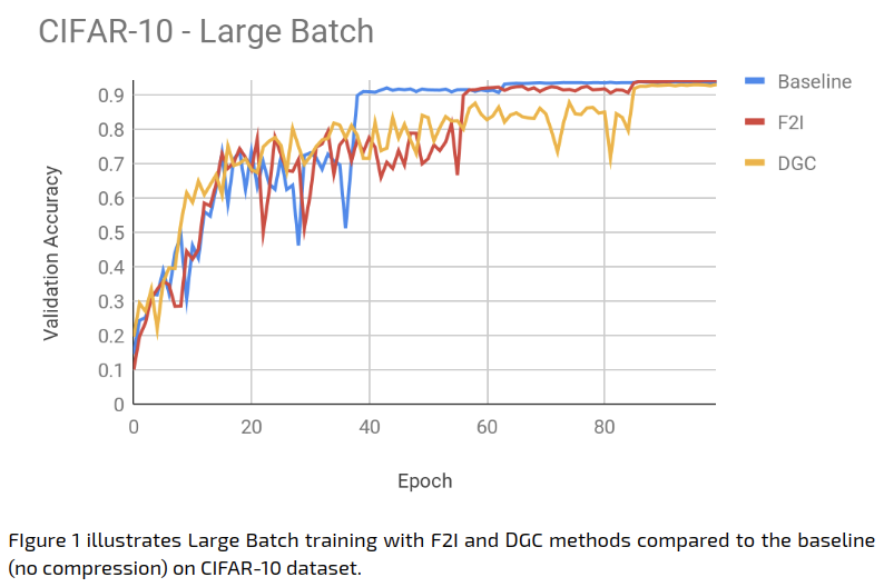
The Large Batch experiment results were as follows:
The learning rate scheduling mechanism that we used in our experiments is ‘reduce on plateau’, which reduces the learning rate when the training loss stops decreasing. It seems, however, that this scheduling is not quite suitable for DGC. As is evident in Figure 1, our experiments suggest that DGC causes a delay in the learning rate reduction, stalling the training process. Other scheduling mechanisms such as cosine annealing [6] may be more suitable, but this requires further research.
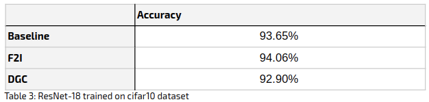
The following table summarizes the accuracy achieved at the end of the training (100 epochs):
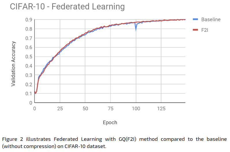
The Federated Learning experiment results were as follows:
The Federated Learning baseline achieves 90% accuracy after 150 epochs, and the GQ applied to the model delta achieves the same accuracy with same number of epochs, with extremely similar behaviour overall.
Communication Effectiveness
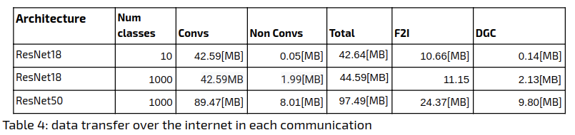
The following table summarizes the compression rates achieved for the various methods. For comparison, we include the ResNet18 and ResNet50 architectures with 10/1000 classes. The number of classes is an additional factor here because as a matter of implementation, DGC sparsifies only the convolutional layers’ parameters and ignores all other parameters, which can be substantial. The dimensions of the fully connected (FC) layer weights are the features length (512/2048 for ResNet18/ResNet50 respectively) times the number of classes. In order to demonstrate the significance of the FC layer we split the original network sizes according to convolutional / non-convolutional layers:
Define the sparsity rate as the percentage of the gradient elements that are not sent. We use sparsity rate warmup (exponentially increasing the gradient sparsity rate from 0.75 to 0.999 during the first 4 epochs).
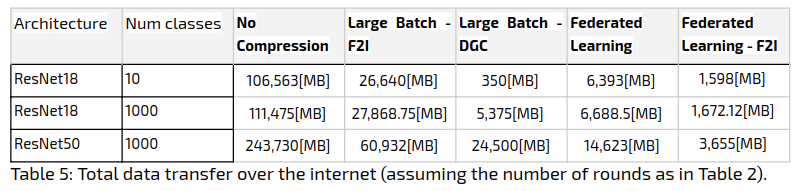
In order to find the amount of data sent to the server in total, we aggregated the data size over the bandwidth. The results appear in the following table:
With respect to total data sent, the Federated Learning approach comes out on top when using 1000 classes: it manages to outperform Large Batch, by a factor of 3. The Large Batch Method with DGC comes out on top when using 10 classes, outperforming Federated Learning by a factor of 5, but requiring additional zip compression on the sparse gradient.
Though Federated Learning a priori requires less communication rounds, Large Batch manages to compete with it in terms of network cost for two reasons:
Higher compression rate (allowing to use DGC over only F2I).
It requires less epochs to converge.
Conclusion
Reducing communication cost is crucial for distributed edge training. As we showed in this post, compression methods can successfully be used to reduce this cost while still achieving the baseline accuracy. We showed how gradient compression methods can be adapted to Federated Learning. In addition, we provided a detailed comparison of the network costs using the different methods presented.
In the next post, we leave aside communications issues, and turn to some complexities related to uneven distribution of data among the devices.