
An Edgify.ai Research Team Publication
In the first post of this series we presented two basic approaches to distributed training on edge devices (if you haven’t read our first post in this series, you should start here). These approaches provide benefits such as AI data privacy and the utilization of the compute power of edge devices. Large-scale distributed training systems, however, may fail to fully utilize that power (as we’ve come to see in our own experiments), as they consume large amounts of communication resources. As a result, limited bandwidth can impose a major bottleneck on the training process.
The two issues described below, pose additional challenges to the general limitation of bandwidth. The first has to do with how synchronized distributed training algorithms work: the slowest edge device (in terms of network bandwidth) “sets the tone” for the training speed, and such devices need to be attended to, at least heuristically. Secondly, the internet connection on edge devices is usually asymmetric, typically twice as slow for upload then for download (table 1). This can severely impede the speed of training when huge models/gradients are sent via the edge devices for synchronization.

Network resources are limited not only by the physical capacity of the underlying fiber/cable that carries the traffic, but also by the processing power and memory of the network devices (these devices/routers are responsible for the difficult task of routing traffic through the network). The network tends to congest when it carries more data than it can handle, which leads to a reduction in network performance (due to TCP packet delay/loss, queueing delays, and blocking of new connections).

Such network restrictions can significantly slow down the training time. In addition, the training must be robust to network failure in order to ensure a stable, congestion-free network. Moreover, in cases where network congestion occurs, the trainer needs to be able to handle it and resume the training process once the network is stable.
There are two main algorithmic strategies for dealing with the bandwidth limitation: (1) Reducing the number of communication rounds between the edge devices and the server (2) Reducing the size of the data transferred in each communication.
1) Reducing communication rounds, as described in the previous post:
Federated Learning is a paradigmatic example for reduced communication. Running Large Batch training requires a communication operation to occur with each batch. Federated Learning, in contrast, runs on the edge device for as many iterations as possible, thus synchronizing the models between the edges as little as possible. This approach is being researched widely in search of ways to reduce communication rounds without hurting accuracy.
2) Reducing the size of the data transferred in each communication, as we now detail in this post. To explain how this can be done, let us first recall the basics of the Large Batch and Federated Learning training methods.
Deep Learning training uses a gradient based optimization procedure for the weights update. A standard procedure for this is Stochastic Gradient Descent (SGD), which can easily be adapted to Large Batch training. Formally, at communication iteration t the following update is performed :

where dW(t) is the average of gradients across all devices and λ is the learning rate. One could also consider the weight update at communication iteration t for Federated Learning. This can be done as follows:

where ΔW(t) is the average of local updates across all devices. Namely, for device i at round t, ΔW(t) is the difference between the initial model for this round W(t) and the final local model Wᵢ(t+1) (the local model that the device sends for averaging at the end of the round). Although the model delta ΔW(t) is not a gradient.
The methods we explored for reducing the amount of data transfer are quantization and sparsification. We can apply those methods to the weights themselves, or to the gradients. We adapt the gradient compression methods to Federated Learning by applying those methods to the weight deltas instead of the gradients.
Gradient quantization (GQ)
GQ is a low precision representation of the gradients, which reduces the data transfer in each communication. So far, there has been limited research on the use of GQ. Some of the known methods of low-precision quantization are 1-bit SGD [1], QSGD [2], and TernGrad [3]. One of the most straightforward methods for quantization is “float32 to int8” (F2I), which reduces the amount of data by a factor of 4. F2I quantization is used widely in the context of inference; this method is integrated in some of the common deep learning frameworks (such as TensorFlow and Caffe) as part of their high performance inference suite. Our experiments show that quantizing the model weights for the training phase is a bad strategy. Quantizing the gradients (GQ), however, does produce good results in training.
Further data reduction can be achieved by using the standard Zip method on the quantized weights. Experiments we’ve conducted reached a reduction of about 50%.
Gradient Sparsification (GS)
Unlike quantization methods, where we try to preserve the information in the gradients with a low precision representation, in GS we try to figure out which parts of the gradients are actually redundant and can be ignored (which can prove to be quite a challenging task). Basic algorithms for GS drop out elements that are smaller than some predefined threshold. The threshold can be predefined before training, or can be chosen dynamically based on the gradient statistics. One such GS method is called “Deep Gradient Compression (DGC)” [4], which is essentially an improved version of “Gradient Sparsification”[5]. In DGC, the threshold is determined dynamically using the gradient statistics. The data that falls below the threshold is accumulated between communication rounds, until it is large enough to be transferred. The threshold is determined by the percentage of data one would like to send, using smart sampling (sampling only 1% of the gradients in order to estimate the threshold). DGC also employs momentum correction and local gradient clipping to preserve accuracy [4].

The Experiments
In our experiments, we have explored the possibility of applying these compression methods to the communication rounds in our two distributed training methodologies without severe degradation of accuracy.
Dataset: CIFAR10, a relatively small, widely used benchmarking dataset. Its 60K data points were split into a training set of 50K and a testing set of 10K data points. (We will present experiments on more substantial datasets in future posts.)
Architecture: Resnet18 (a common deep learning architecture). Training was done from scratch (no pre-training).
Optimizer: SGD
Distributed setting: The training process was distributed across 32 virtual workers (with a single K80 GPU for each worker). The training data for this experiment was distributed in an even (IID) fashion.
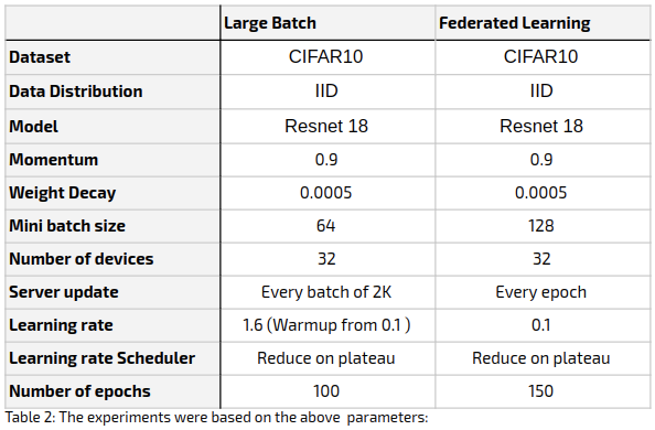
All experiment parameters are as detailed in the table below.

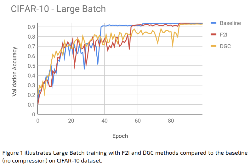
The Large Batch experiment results were as follows:

The learning rate scheduling mechanism that we used in our experiments is ‘reduce on plateau’, which reduces the learning rate when the training loss stops decreasing. It seems, however, that this scheduling is not quite suitable for DGC. As is evident in Figure 1, our experiments suggest that DGC causes a delay in the learning rate reduction, stalling the training process. Other scheduling mechanisms such as cosine annealing [6] may be more suitable, but this requires further research.
The following table summarizes the accuracy achieved at the end of the training (100 epochs):

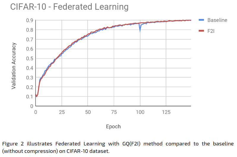
The Federated Learning experiment results were as follows:

The Federated Learning baseline achieves 90% accuracy after 150 epochs, and the GQ applied to the model delta achieves the same accuracy with same number of epochs, with extremely similar behaviour overall.
Communication Effectiveness
The following table summarizes the compression rates achieved for the various methods. For comparison, we include the ResNet18 and ResNet50 architectures with 10/1000 classes. The number of classes is an additional factor here because as a matter of implementation, DGC sparsifies only the convolutional layers’ parameters and ignores all other parameters, which can be substantial. The dimensions of the fully connected (FC) layer weights are the features length (512/2048 for ResNet18/ResNet50 respectively) times the number of classes. In order to demonstrate the significance of the FC layer we split the original network sizes according to convolutional / non-convolutional layers:

Define the sparsity rate as the percentage of the gradient elements that are not sent. We use sparsity rate warmup (exponentially increasing the gradient sparsity rate from 0.75 to 0.999 during the first 4 epochs).
In order to find the amount of data sent to the server in total, we aggregated the data size over the bandwidth. The results appear in the following table:

With respect to total data sent, the Federated Learning approach comes out on top when using 1000 classes: it manages to outperform Large Batch, by a factor of 3. The Large Batch Method with DGC comes out on top when using 10 classes, outperforming Federated Learning by a factor of 5, but requiring additional zip compression on the sparse gradient.
Though Federated Learning a priori requires less communication rounds, Large Batch manages to compete with it in terms of network cost for two reasons:
- Higher compression rate (allowing to use DGC over only F2I).
- It requires less epochs to converge.
Conclusion
Reducing communication cost is crucial for distributed edge training. As we showed in this post, compression methods can successfully be used to reduce this cost while still achieving the baseline accuracy. We showed how gradient compression methods can be adapted to Federated Learning. In addition, we provided a detailed comparison of the network costs using the different methods presented.
In the next post, we leave aside communications issues, and turn to some complexities related to uneven distribution of data among the devices.
